PROBLEM SET 5 - IS-LM AGGREGATE DEMAND

AGGREGATE SUPPLY MODEL - ANSWERS

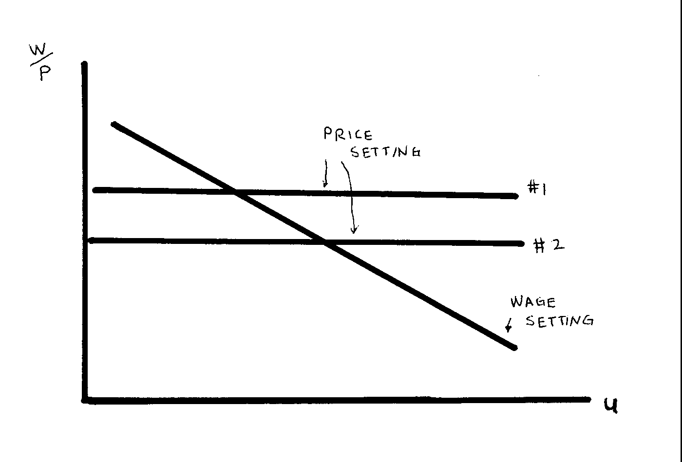
1. To determine the answer we need to equate the real wage (W/P) implied by the price setting equation with the real wage implied by the wage setting equation and solve for u.

Price Setting Equation - P = 1.1 W (this gives a markup of 10%)

Wage Setting Equation - W = P(1-u)

From the price setting equation we get W/P = 1/1.1 = .9090909

From the wage setting equation we get W/P = 1-u

Setting these two equal yields .9090909 = 1-u. Solving for u gives

u = .090909

2. The derivation above is changed by amending the price setting equation to

P = 1.2 W, which yields W/P = .833333, and following the same pattern as above yields:

u = .166666

The graph shows that the price setting equation shifted from W/P = 1/(1+m) = .90909 to .83333. In this model the wage setting equation is linear.

3. The level of unemployment benefits are one of the variables captured in z in the wage setting equation W = P F(u,z). An increase in unemployment benefits will increase z and shift the function up in the W/P plane. To understand this reason as follows: with higher unemployment benefits at each level of unemployment it will take a higher real wage to entice workers to accept employment (in other words workers have more bargaining power). An upward shift in the wage setting equation will lead to a higher natural rate of unemployment - hence more generous unemployment benefits could be part of the explanation of higher unemployment in European countries.

4. A higher multiplier means a flatter IS curve (because for a given change in i which causes a given change in I a bigger multiplier means a bigger change in Y). A flatter IS curve means that there will be a flatter AD curve.

5. Smaller markups mean a smaller natural rate of unemployment (see the comparison between #1 and #2 above). With a smaller natural rate of unemployment, the natural level of income, Y_n, will be higher. The point P^e, Y_n will shift to the right, and the whole AS curve will shift as well.

6. A vertical LM curve (which might result from the interest sensitivity of Money Demand being zero) would still shift with changes in the price level, so the AD curve would still be a downward sloping curve. However, a shift in the IS curve would not shift the AD curve.

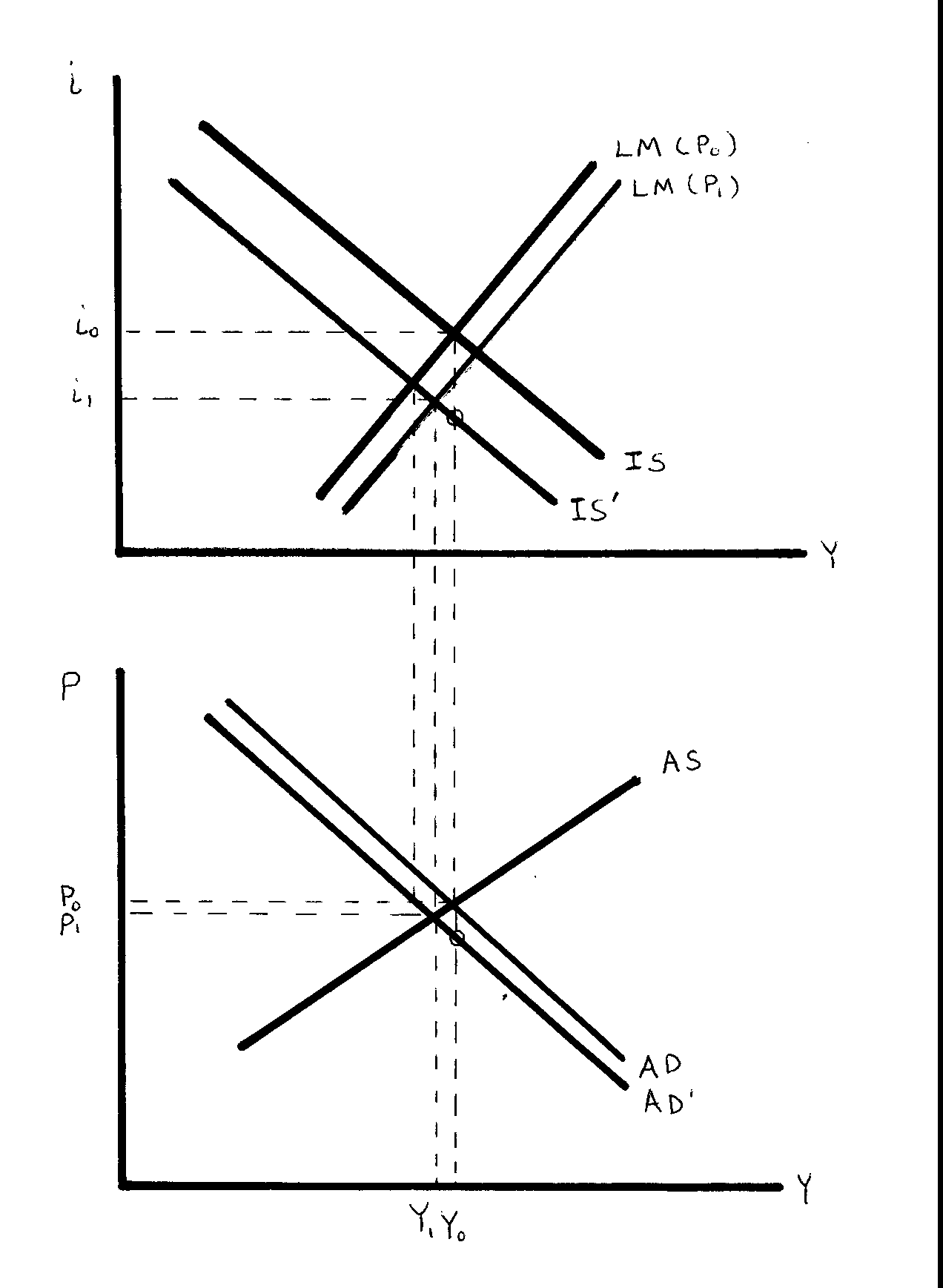
7. See the figure to verify the following results:

Y i P

Short Run dn dn dn

Long Run noD dn dn

The tax increase causes a shift in the IS curve to IS'. This IS shift causes a shift in the AD curve to AD'. In the short run i goes to i₁, P goes to P₁, and Y goes to Y₁. In the long run the circled points prevail.

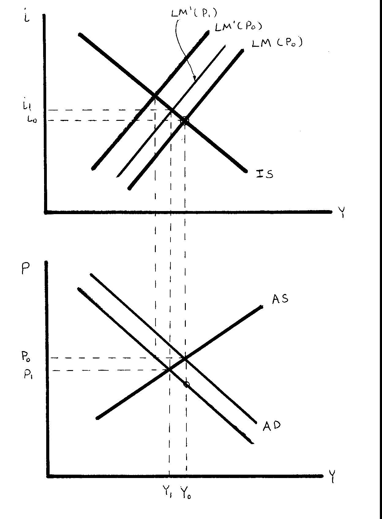
8. See the figure to verify the following results:

Y i P

Short Run dn up dn

Long Run noD noD dn

The decrease in the money supply causes a shift of the LM(P₀) to LM'(P₀). This LM shift causes a shift in the AD curve to AD'. In the short run i goes to i₁, P goes to P₁, and Y goes to Y₁. In the long run the circled points prevail.

9. If P^e > P, then we can expect P^e to fall, and that will cause the AS curve to fall. A falling AS curve will mean falling prices and increasing incomes.

10. There are many comments one could make. First, in the long run we are all dead, so who cares about the long run? Second, the short run might be a long time and waiting around for the long run adjustments may put the world through more pain than is needed. We will talk about this type of thing much more later in the course.